Poisson Solvers
A suite of efficient solvers for self-gravity in 2D/3D
Introduction:
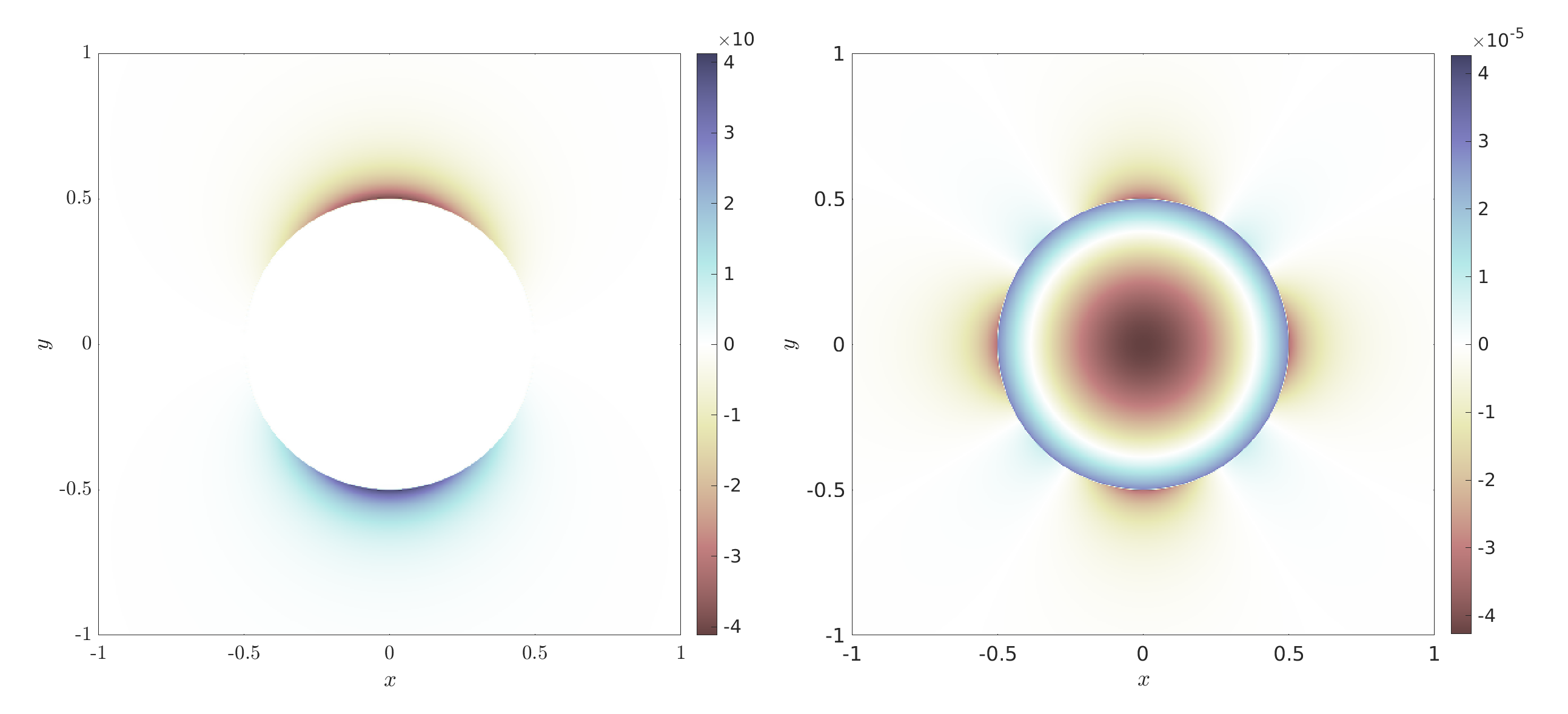
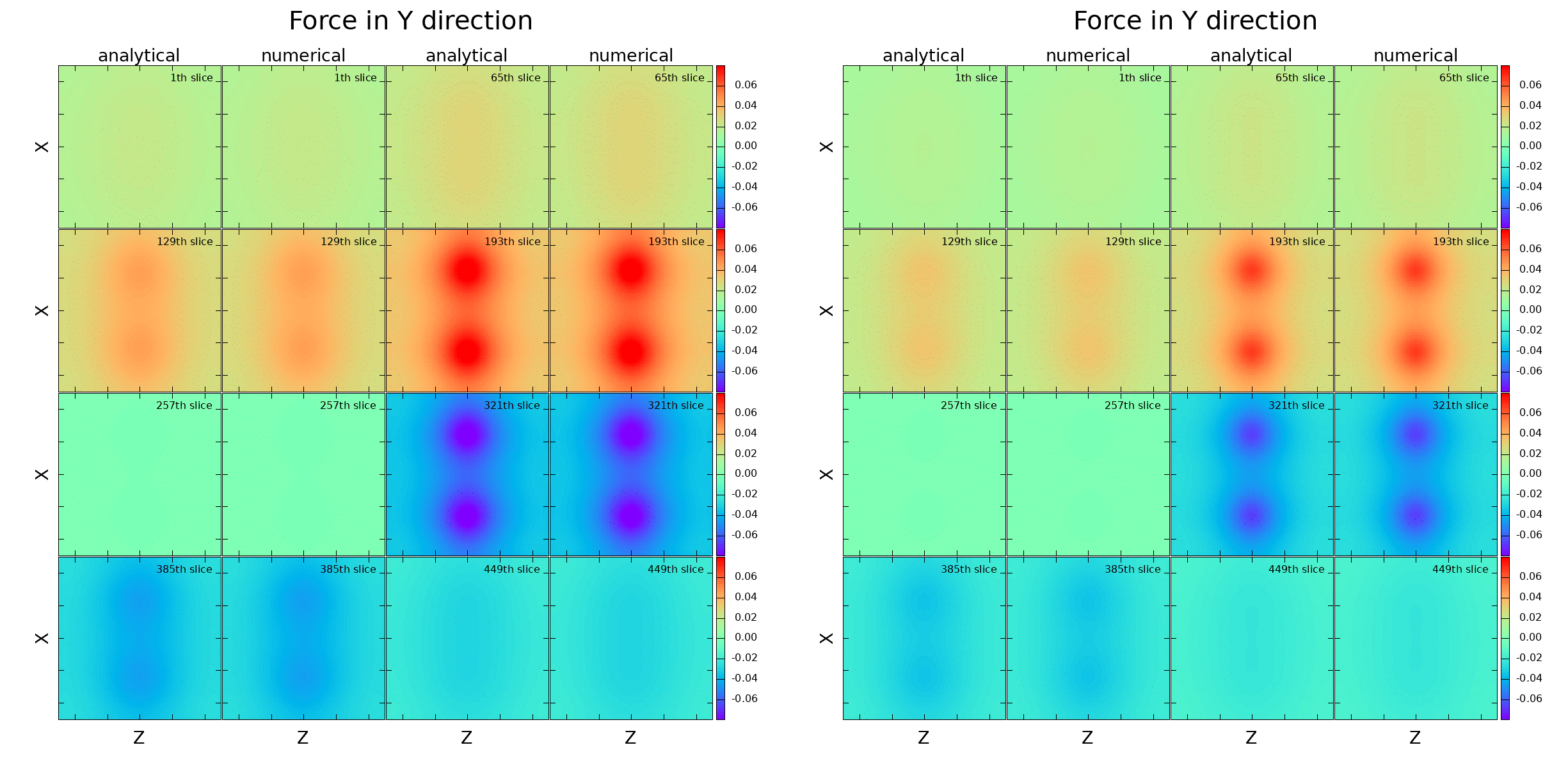
We develop a suite of efficient solvers to compute self-gravity in 2D and 3D, including accurate direct methods using open or isolated boundary conditions, natural in astrophysics. The forces are represented as the convolution of the derivative of the Poisson kernel and the density. The numerical method employs the Taylor expansion for the density and analytical calculation on the product of polynomials and the kernel to retain high accuracy. The discretized sum is set in convolution form. The numerical complexity for direct calculation is O(N⁴) and O(N⁶) for 2D and 3D, respectively. By means of the Fast Fourier Transform applied to sums in convolution form, the high computational complexity otherwise associated with direct methods is reduced to O(N³ logN³) in 3D; alternatively or concurrently, GPU computing can also reduce computational costs. The direct methods require specific grid structures; suite development progressively widens the applicability range.
Development of Poisson Solvers:
We have already developed solvers for many practically important cases, such as
- Cartesian uniform grids in 2D (Yen et al. 2012) and 3D (Krasnopolsky et al. 2021, figures below)
- Cartesian nested grids in 2D (Wang et al. 2016), 2D polar with logarithmic radius (Wang et al. 2015)
- Cartesian spline functions in 2D (Wang et al. 2019), multi-grid in 2D and 3D (Wang & Yen 2020).
- GPU generalization to AMR grids in 2D was advanced in Tseng et al. (2019).
- Currently, we develop solvers for Cartesian nested/AMR grids in 3D, and higher order of accuracy in 3D will be considered.
Gallery